
Global Mangrove Watch puts Pakistan's mangroves at 738 square kilometres in 2020. A dataset built at the Institute of Space Technology in Islamabad, by Gilani and colleagues, maps 1,337 square kilometres in the same year across five sites that hold nearly all of them. Other figures in circulation run to about 2,400. All rest on satellite imagery, but they are not measurements of one thing. Figure 1 shows that they differ in the year they refer to and the coast they cover as well as in method, and the largest, a Sindh Forest Department figure stated in 2024, carries no reference year. The comparison this notebook can make properly is between the first two.
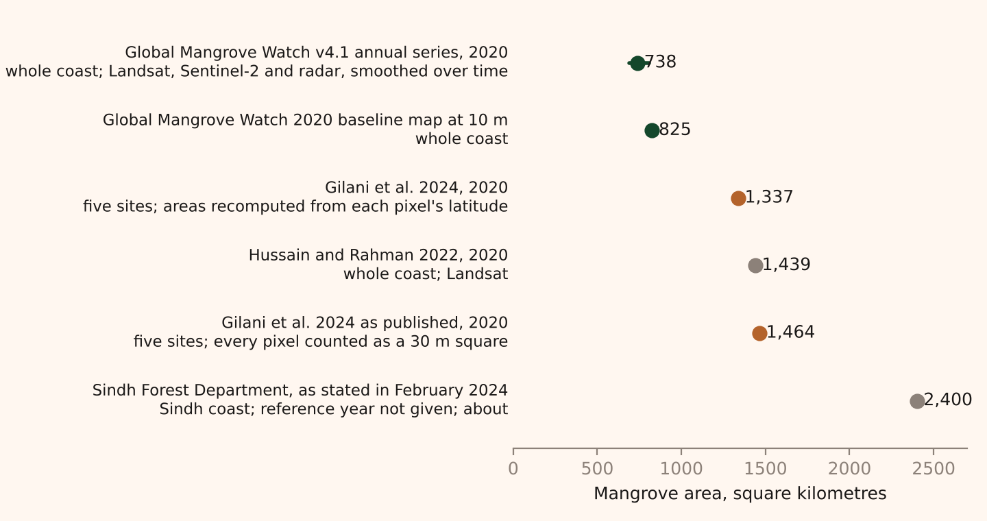
A satellite map of mangroves is not a photograph with the trees counted. It is a classification: a rule, or a trained model, that reads the light reflected from each patch of ground and decides whether that patch is mangrove, water or something else. The total is the number of patches the rule accepted, multiplied by the area of a patch. Each part of that sentence can be done differently, and the figures in Figure 1 differ partly because the parts were. The Indus delta, where more than 95 per cent of Pakistan's mangroves stand, is the case throughout. Adaad holds two records of it. The Gilani dataset maps five sites every five years from 1990 to 2020, and Global Mangrove Watch maps the whole coast every year from 1985 to 2025. Both are free to reuse, and both are described more fully in the method note.
A pixel is thirty metres, except when it is not
The Landsat satellites, which both records rely on for most of their history, see the ground in squares 30 metres on a side. Everything inside a square is averaged into one set of numbers, one for each colour band the sensor records. A single mangrove tree is invisible. A stand 100 metres across is about three pixels wide, and its edge is a row of pixels that are partly tree, partly mud and partly water. Sentinel-2, which Global Mangrove Watch uses for its 2020 map, sees 10 metre squares, so the same stand is ten pixels wide, the edge gets sharper and the count of mixed pixels falls, but the problem does not go away.
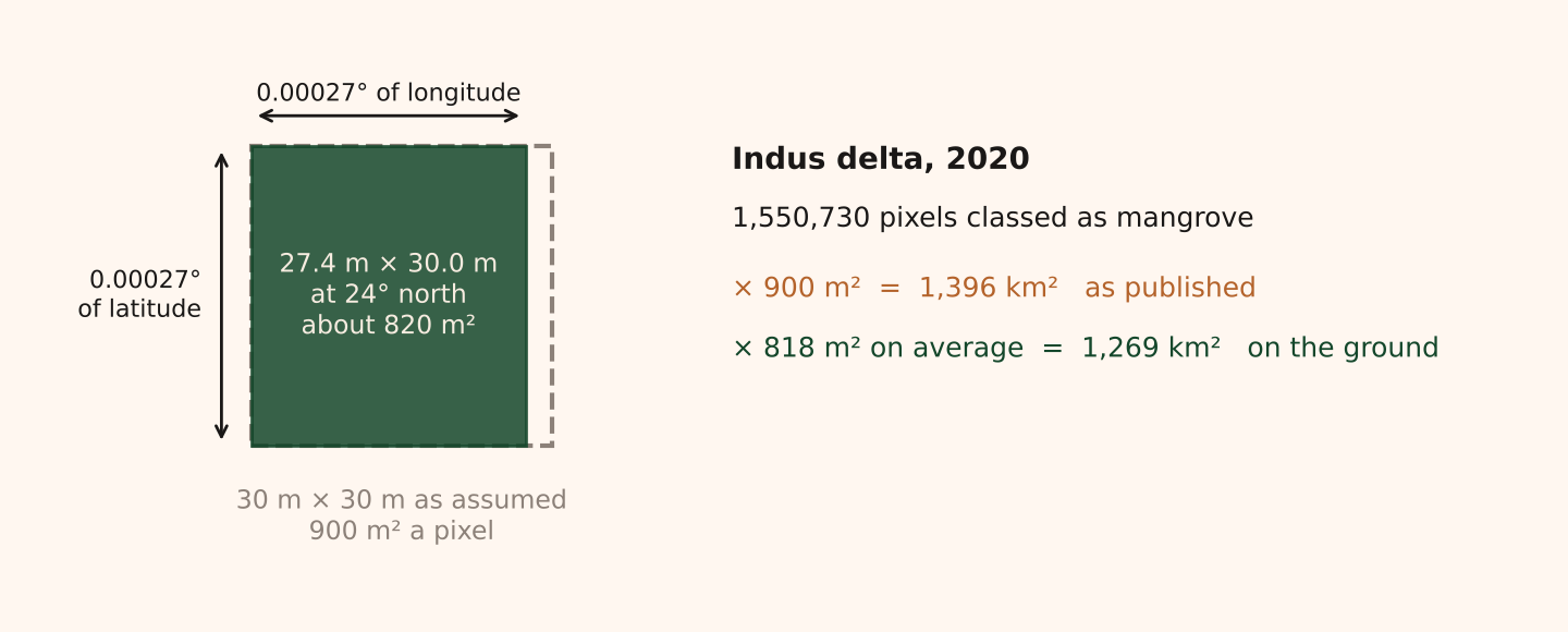
The area of a pixel sounds like the one fixed quantity in the chain. It is not. The Gilani maps of the Indus delta are stored on a grid of latitude and longitude, 0.00027 degrees a side. A degree of latitude is about 111 kilometres everywhere, so the pixel is 30.0 metres tall. A degree of longitude shrinks towards the poles, and at 24 degrees north it is 102 kilometres, so the same pixel is 27.4 metres wide. The dataset's attribute table multiplies its pixel counts by 900 square metres, the area of a true 30 metre square. The 1,550,730 delta pixels classed as mangrove in 2020 then come to 1,396 square kilometres. Multiplied by the pixel's area on the ground, which averages 818 square metres across the delta, they come to 1,269. Figure 2 draws the difference. Recomputing the pixel area reduces the published total by about 9 per cent, and the four smaller sites, which are stored on a metric grid, have no such gap. Adaad's figures in this notebook use the recomputed areas; the published ones are shown alongside where the comparison matters.
What the sensor sees
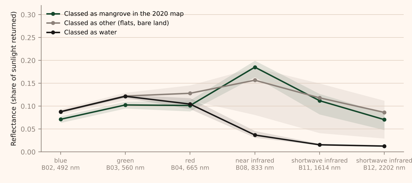
A sensor records how much sunlight each patch of ground reflects in each of several bands of the spectrum. Healthy leaves reflect strongly in the near infrared, just beyond the red that eyes can see, and absorb red light for photosynthesis, so vegetation is bright in one band and dark in the other. Water absorbs the near infrared almost completely. Wet mud sits between the two. Figure 3 shows these signatures in a Sentinel-2 scene of the creeks east of Keti Bandar taken on 29 October 2026, with the pixels sorted by what the Gilani map called them in 2020. Water falls away after the red band. Mangrove and bare flat run close together in the visible bands and separate in the near infrared, where the pixels classed as mangrove return 0.19 of the sunlight and the flats 0.16. The gap is narrow. That is consistent with the 2020 class here including sparse cover with mud between the plants, but a 2026 scene cannot separate that from change since 2020, the tide on the day or errors in the map.
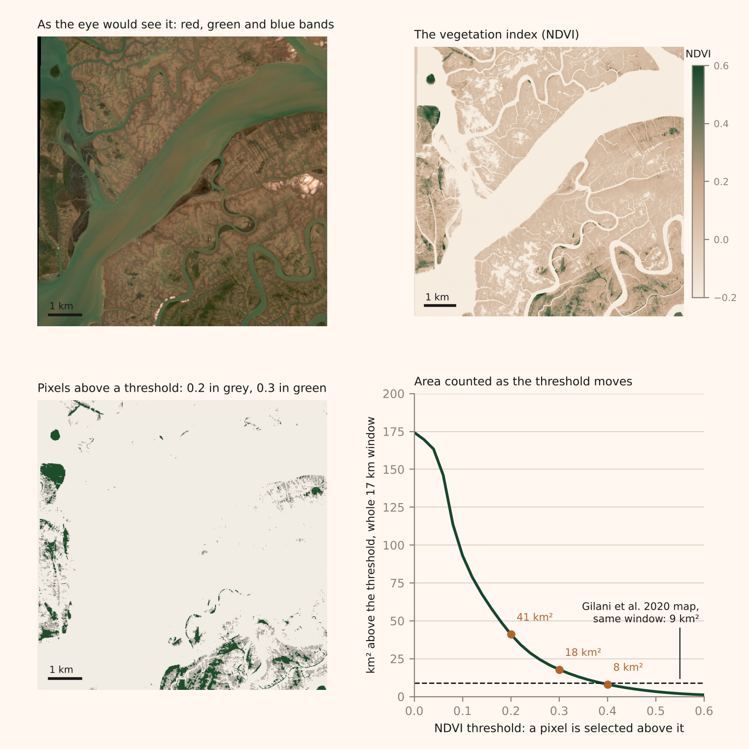
The simplest rule for finding mangroves draws a line through that space and calls everything on one side mangrove. The usual line is a vegetation index, the difference between the near infrared and red bands divided by their sum, which runs from about minus one for water to plus one for dense leaves, and a threshold on it. Where the threshold goes decides the area. Figure 4 applies three to the same scene. Above 0.4 the window holds 8 square kilometres; above 0.3 it holds 18; above 0.2 it holds 41. Those are areas above a threshold, not areas of mangrove. The index responds to vegetation greenness; it does not identify the plant or establish that it is growing in tidal water, so the green may be mangrove, salt marsh or algae on wet mud. The 2020 map puts 9 square kilometres of mangrove in the same window, six years earlier, which the strict threshold matches and the loose one exceeds by four and a half times. A strict rule misses the sparse and young stands at the seaward edge, which in a spreading forest is where the growth is. A loose rule catches them, and also catches things that are not mangrove and the mixed pixels along every creek. Choosing the rule, and then checking it, needs reference observations: places on the ground, or in imagery sharp enough to stand in for the ground, where someone has recorded what is actually there.
Choose the threshold and see what the map counts
The image is the Sentinel-2 window east of Keti Bandar on 29 October 2026, 17 kilometres across. Every pixel with a vegetation index above the threshold is coloured, and the colour shows whether the 2020 map also classes that ground as mangrove.
The picture is drawn at a quarter of the scene’s resolution; the areas are counted at full resolution. Source: Copernicus Sentinel-2 L2A, 29 October 2026; Gilani et al. 2024; Adaad calculations.
The tide moves the line too. At low water a sparse stand on a mudflat reads as vegetation over mud; at high water the same stand reads as vegetation over water, or as water with a little green in it. A map built from scenes taken at different states of the tide sees different forests at different dates, and a map built from a composite of many scenes sees an average tide that never happened. Season matters in the same way. The two records in this notebook use different scenes, different composites and different rules, and nothing in their published descriptions allows the three effects to be separated.
From a rule to a classifier
Neither record draws a single line. Gilani and colleagues trained a random forest, an ensemble of decision trees, on Landsat scenes, using points the analysts labelled by eye as mangrove, water or other, and produced one map for each of seven years. A classifier of this kind is a threshold in many dimensions rather than one, and what it learns is what its training points teach it. If the labelled mangrove points are mostly closed canopy, the classifier learns closed canopy, and the sparse edge is classed as other.
Global Mangrove Watch works in more stages, set out in the method note. It combines optical imagery with radar, which sees the structure of a canopy rather than its colour, and filters each pixel's result over time, so that a pixel which is mangrove in 2014 and 2016 is unlikely to be read as something else in 2015. The record reports a global F1 score of 0.93, a single number that combines two rates: about 6 per cent of true mangrove missed and about 8 per cent of mapped mangrove wrong. It is not the share of pixels classified correctly, and it is a figure for the world, not an error bar for Pakistan. The record's authors also say that usable imagery thins out before about 2000, so its earlier values rest more on infilling from the years around them.
Figure 5 puts the two records on one chart. In 1990 they agree: 436 square kilometres in the Gilani maps, 407 in Global Mangrove Watch, and the first sits inside the second's own 95 per cent range. From 2000 the gap opens. By 2020 the Gilani total is 1,337 square kilometres and Global Mangrove Watch is 738, with a range of 688 to 808. The records therefore disagree on the growth as well as the level: 206 per cent over thirty years in one, 81 per cent in the other. The candidate reasons are the ones above, and none has been tested. Global Mangrove Watch's training data are global and its time filter smooths the series. The Gilani classifier was trained on Pakistani points and may accept sparser cover. Both are model outputs, and averaging them would produce a third number that no model made.
Boundaries
The Gilani dataset covers five delimited sites: the Indus delta, Sandspit at Karachi, and Miani Hor, Kalmat Khor and Jiwani on the Balochistan coast. Its Indus delta raster ends at 68.76 degrees east, which is short of Badin's coast, where Delta Blue Carbon, the mangrove planting and restoration project in the delta, is planting its second phase. Any mangrove there is in Global Mangrove Watch's national total and not in the five site total, so the two records are not even measuring the same stretch of coast. The site total is close to a national one, because almost all of Pakistan's mangroves are in the delta, but it is a lower bound for Badin and it is zero for any creek the site polygons missed.
District figures carry a rule of their own. Mangroves grow seaward of the coastline that the district boundaries follow, so a district total has to decide what to do with pixels that fall in no district. Adaad gives each such pixel to the nearest district. That rule accounts for 14 per cent of Thatta's figure and 80 per cent of Lasbela's, whose mangroves are in a lagoon. A different rule, or a different coastline, gives different district totals from the same raster.
A map of change is two maps subtracted
A growth figure is the difference between two classified maps, and it inherits the errors of both. Figure 6 breaks the Gilani series down for the two districts that hold most of the delta's mangroves, Thatta and Sujawal, step by step from 1990 to 2020. Each bar is the area classed as mangrove at the end of a five year step, split into what was already mangrove in the earlier map and what is new. Below the line is what the earlier map called mangrove and the later map does not.
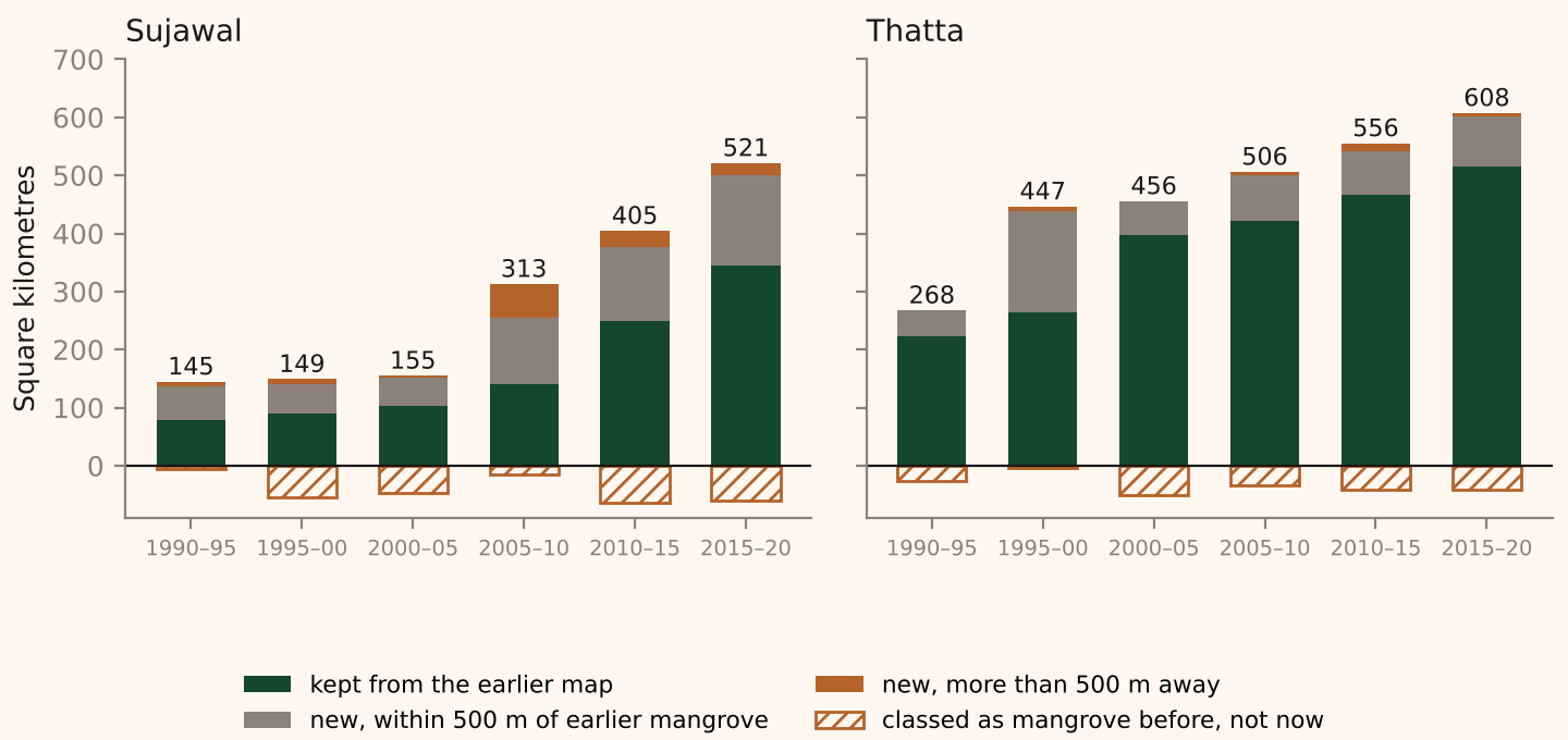
Sujawal's mapped area goes from 155 square kilometres in 2005 to 313, 405 and 521. Between 2015 and 2020 it gained 177 square kilometres and lost 61, and Thatta gained 93 and lost 40. Between 1995 and 2000 Sujawal lost 55 square kilometres from its mapped mangrove and gained 60 elsewhere: about 62 per cent of the earlier mapped forest remained, while the net total changed by only 4 square kilometres. The maps do not say what the losses are. They may be real change, a different tide or month in the scene, or the classifier placing the same ground on the other side of its threshold, and the analysis here does not separate the three. What Figure 6 does show is that a net growth figure can hide a much larger gross turnover.
Global Mangrove Watch's time filter is designed to damp such turnover, which is why its series is smooth, and the cost is that a real change in one year is spread over the years around it. Its growth steps up around 2007, from 5 square kilometres a year over 1990 to 2006 to 18 a year over 2006 to 2015 and 18 again over 2015 to 2025, with the caution that its values before 2000 lean on infilled years. The Gilani snapshots show bursts in 1995 to 2000 and 2005 to 2010, each of about 44 square kilometres a year. The two records do not agree on when the forest grew fastest, and neither pins the date closely. Delta Blue Carbon began planting in 2015. In Global Mangrove Watch the growth rate after 2015 is no higher than in the eight years before it. That is a fact about two series, not a finding about the project.
Is Sujawal's jump real?
Sujawal's mapped mangrove grew by 366 square kilometres between 2005 and 2020, net of losses, which is two thirds of the 551 square kilometres the five sites gained together, and the district has no second source: Global Mangrove Watch publishes a national series, not a district one. The classified maps can be questioned on their own terms. A forest that spreads outward from existing stands adds pixels next to pixels that were already mangrove. New stands on bare flats, whether planted or seeded by the tide, appear away from the old ones. A classifier that has started to accept something new, such as salt marsh or algal mats, adds pixels wherever that something is. The distance from each new pixel to the nearest pixel that was already mangrove separates the first pattern from the other two.
Figure 7 maps it. Of the 388 square kilometres classed as new mangrove in Sujawal between 2005 and 2020, before the 22 that the 2005 map had and the 2020 map lost, 164 lies within 500 metres of mangrove mapped in 2005, 131 lies between 500 metres and 2 kilometres away, and 93 lies more than 2 kilometres from any of it. In Thatta the shares run the other way: 136 of its 193 square kilometres of new mangrove, 71 per cent, is within 500 metres of the earlier stands. Almost all of the new mangrove in both districts was classed as other, not water, in 2005, so the pixels that became mangrove were bare or sparsely covered land, not open channels that silted up. In Sujawal 157 square kilometres sits in patches that contain no 2005 mangrove at all, and 21 of those patches are a square kilometre or more. The three largest, each above 5 square kilometres, are ringed on the map.
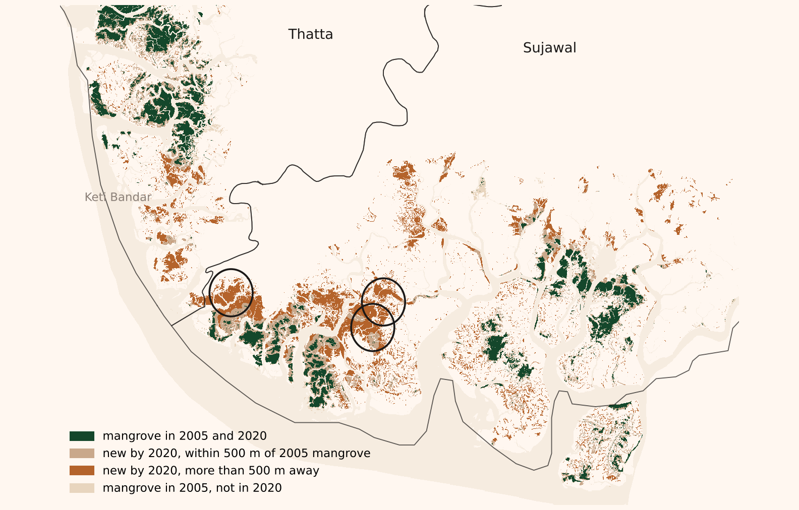
The pattern says that Sujawal's growth did not come mainly from the edges of its old stands. It does not say what produced it: planting, natural colonisation of flats that the river's shifting channels have left at the right height, or a classifier reading sparse growth, or something that is not mangrove, as forest.
High resolution imagery of the three ringed patches narrows this without settling it. The first was a bare flat in February 2003, carried clumps of small dark plants and straight bund lines in January 2013, and by December 2023 was open scrub with mud visible between the plants. It was not viewed near 2020, when the map calls 93 per cent of the window mangrove. The second had scattered shrubs along its creeks in January 2011 and was still mostly bare in May 2020, with lines of vegetation along creeks and dykes; the map calls 37 per cent of it mangrove. The third had scattered shrubs in January 2011 and denser cover on both banks of its creek in May 2020, which had thickened further by January 2023; the map calls 85 per cent of it mangrove. Vegetation spread at all three, and the views are consistent with the map including sparse cover. They do not establish it: the dates only partly match the map's, the views have not been matched to the classified pixels, Global Mangrove Watch has not been read at the same places, and a view from above does not confirm that a plant is a mangrove. Bunds and vegetation along dykes are the kind of marks planting leaves, but seedlings carried in by the tide settle along the same lines. Three things remain uncertain: whether each new pixel is mangrove, how dense the cover is, and why it appeared. Sujawal's 521 square kilometres rests on one classifier's answer to the first two, and neither record answers the third.
The questions to ask
Six steps separate a satellite image from a sentence that says mangroves cover so many square kilometres. They are the size and shape of the pixel, the bands the sensor sees, the rule or model that assigns a class and what it was trained on, the date and tide of the scenes, the arithmetic that turns pixels into area, and the boundary within which they are counted. In this notebook the pixel's shape moved the delta's figure by 9 per cent on its own, and the two records, which differ in training data, imagery, smoothing and the stretch of coast they cover, end a factor of 1.8 apart; the notebook cannot say how much of that gap each step contributes. A reader who meets a satellite figure for anything, forest, flood, cropland or solar panels, can ask which of the six produced it and whether the author says.
The solar capacity estimates in this issue's Big Read come from the same kind of pipeline at the other end of the resolution scale, where a home's array is a fraction of one Sentinel-2 pixel and the model reads a roof's colour rather than outlining a shape. The published ranges, there and for Global Mangrove Watch's 688 to 808, account for specified uncertainties within each estimation method. They do not necessarily cover systematic error from the choice of training data, definition or model, and that is the uncertainty the six questions are for.
Sources. Gilani, H., and colleagues, Mangrove Cover Dataset of Pakistan 1990–2020, Zenodo, version 1, March 2024, CC BY 4.0, from the Institute of Space Technology, WWF and the Sindh Environmental Protection and Mangrove Watch Alliance; the method is described in Gilani et al., Estuarine, Coastal and Shelf Science, 2021. Global Mangrove Watch version 4.1.12, annual extent 1985–2025, Bunting, Hilarides, Rosenqvist and colleagues, Zenodo, 2026, CC BY 4.0; the Pakistan row of its country statistics workbook, checked against the series served on the Global Mangrove Watch site. Hussain and Rahman, Monitoring spatial and temporal distribution, pattern, and trend prediction of coastal mangroves in Pakistan using geospatial techniques, in Science for Sustainable Societies, Springer, 2022, give 48,331 hectares in 1986 and 143,930 in 2020 from Landsat. The Sindh Forest Department's figure of about 240,000 hectares is as given by Shehzad Sadiq Gill, a divisional forest officer, to Mongabay in February 2024, which also quotes the department's 80,000 hectares for 1990; other departmental figures in circulation are 210,000 hectares for 2020 and 250,000 for 2021. These are shown for comparison only. District boundaries are the 2023 census frame.
Imagery. The Sentinel-2 scene is Level 2A surface reflectance for 29 October 2026, tile 42R, cut to a 17 by 16 kilometre window between 67.46 and 67.63 degrees east and 23.99 and 24.14 degrees north, bands 2, 3, 4, 8, 11 and 12 at 9 metres in UTM zone 42, downloaded from the Copernicus Browser; the sensor passes at about 10.50 local time and the flats in the scene are largely exposed. The vegetation index is (B08 minus B04) over (B08 plus B04). Reflectance by class in Figure 3 is the median over pixels of the Gilani 2020 map resampled onto the scene's grid, with the middle half shaded. The high resolution views are Google Earth's historical imagery at the three patch centroids, 27 February 2003, 8 August 2009, 15 January 2013 and 11 December 2023 for the first, 6 January 2011, 6 May 2020 and 12 January 2023 for the second and third; they were used to check the classification and are not reproduced.
The two classifiers. Gilani and colleagues ran a random forest on Landsat imagery in Google Earth Engine with three classes, trained on points labelled from high resolution imagery. Global Mangrove Watch classifies Landsat and Sentinel-2 imagery for a set of baseline years with a gradient boosted model trained on its own 10 metre map of 2020, runs a random forest for every year, merges the result with L-band radar from Japan's satellites into a probability for each pixel, filters the probabilities over time and applies a threshold.
Areas. The Gilani Indus delta rasters are in geographic coordinates with pixels of 0.000269 degrees. Area is recomputed for each row of pixels from its latitude, on a spherical Earth of radius 6,371.0 kilometres: the pixel's height and width in radians, multiplied by the radius squared and the cosine of the row's latitude. The same formula is used for the national, district and change figures. It gives 1,269 square kilometres for the delta in 2020 against the 1,396 in the dataset's attribute table and 1,337 for the five sites against 1,464. The four other sites are in UTM projections with true 30 metre pixels and match their tables. All figures in the text use the recomputed areas unless marked as published.
Change and distance. Each earlier map is resampled onto the 2020 grid by nearest neighbour; the grids differ by a few pixels in extent. Figure 6 covers all six five year steps from 1990. Sujawal's 2005 to 2020 change is 388 square kilometres classed as new and 22 classed as lost, a net gain of 366, from 155 to 521, which matches the district table in Adaad's mangrove dataset. New mangrove in a step is any pixel classed as mangrove in the later map and not in the earlier one; lost is the reverse. Distance is measured from each new pixel to the nearest pixel classed as mangrove in the earlier map, in pixels, converted at 28.5 metres a pixel. A patch is a group of mangrove pixels connected edge to edge in the 2020 map, and a patch is counted as new when it contains no pixel classed as mangrove in 2005. District totals in Figure 6 assign every pixel, offshore included, to the nearest 2023 district polygon; they differ slightly from the district table in Adaad's mangrove dataset, which treats Karachi's districts separately, so Thatta reads 608 square kilometres here against 576 there. The code and the tables are in the notebook's exercise folder.
What is not done. The two records are not compared pixel by pixel, because Global Mangrove Watch's Pakistan rasters have not been pulled, so the imagery check says nothing about what that record calls the same ground. The mapped losses have not been inspected in imagery. The threshold exercise in Figure 4 is a demonstration on one scene from 2026 against a map from 2020; it is not a reproduction of either record's method, and the window holds only 9 square kilometres of mapped mangrove, so its percentages are not the delta's.
Data and methods downloads
- Global Mangrove Watch annual extent for Pakistan, 1985–2025, with 95 per cent range (CSV)
- Gilani et al. site areas every five years, 1990–2020, recomputed and as published (CSV)
- The two records side by side, 1990–2020 (CSV)
- Gains, losses and distance from earlier mangrove by district and step (CSV)
- Patches of 2020 mangrove with no 2005 mangrove, 0.5 km² and over, with centroids (CSV)
- New mangrove in Sujawal and Thatta by distance from 2005 mangrove, every 50 metres (CSV)
- Area above each NDVI threshold in the Sentinel-2 window, and the part the 2020 map classes as mangrove (CSV)
- Gilani et al., Mangrove Cover Dataset of Pakistan 1990–2020 (Zenodo) ↗
- Global Mangrove Watch v4.1 (Zenodo) ↗
- Copernicus Browser (Sentinel-2) ↗
- Hussain and Rahman 2022 (Springer) ↗
- Source and method notes (Markdown)